Assignment 5: Processing Pix4D Imagery with GCPs

Introduction

For this assignment the objectives were to further learn about how to process imagery in Pix4D, use Pix4D's rayCloud GCP editor, rematch and optimize the imagery, and merge two projects into one DSM and orthomosaic rendering.

This assignment involved using a lot of the same methods as the last image processing assignment, however this time GCPs were used. A GCP or ground control point, is a physical landmark that represents a known coordinate. These markers are placed at various ground locations throughout the site of study. When the UAS is in flight, it takes aerial photographs of the ground and in those photographs, some will contain GCPs. When the user goes to process the imagery, the ground control points are used to georeference the locations of the photographs, placing the imagery into a coordinate system.

Methods

For this assignment, the two Litchfield flights were processed separately, but the same methods were applied to both. The first step was to process the Litchfield flight 1 photos. The same methods used to process imagery in Assignment 3, were used in this processing. Before initially processing the images, however, a file containing the GCP coordinates was added to the map.

Figure 1: Adding GCPs before initial processing 

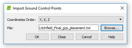
Figure 2: Importing .txt file containing GCP coordinates  

Figure 3: Map view after GCPs were added to the map (from Flight 2 processing)

Once this was done and initial processing was complete, the GCPs were tied down using the rayCloud GCP editor. Figure 4 shows the GCP locations as floating blue points in the rayCloud.

Figure 4: Pre-GCP editing

Obviously, floating GCPs aren't exactly what's desired for tying down the images, so the next step was to use the rayCloud GCP editor and match all the floating points with their corresponding GCPs, using the aerial photographs.

Figure 5: Using the rayCloud GCP editor

Once the floating GCP point was clicked on, the user could find the actual GCP in the images containing it and clicked on the center to accurately tie down the floating point to its corresponding GCP, thus georeferencing the images. After all floating points were tied down to GCPs, the project was rematched and optimized. In figure 6 and figure 7, the green points represent the tied down GCP locations. The blue points in figure 7 represent speculated GCP locations that were not found in any of the images during GCP editing. 

Figure 6: rayCloud before imagery has been rematched and optimized

Figure 7: rayCloud view of rematched and optimized project (flight 2)

 When looking at figure 7, the green triangles represent the height and position of the photos from the initial flight and the blue triangles represent the corrected position and imagery after rematching and optimizing. From there, the rest of the processing was completed and the quality report, DSM, and orthomosaic rendering were produced. Then, the same processes were done for the Litchfield flight 2 images.

Figure 8: Summary and preview of Litchfield flight 1 from quality report.

Once both flights were processed, they were merged together by going through yet another full processing. The final result? A fully rendered DSM and orthomosaic of the entire Litchfield mine.

Results

As compared to processing imagery with out GCPs.

Figure 9: Merged DSM Hillshade

Figure 10: Comparison Hillshade DSM

Looking at figure 9 and figure 10, figure 9 shows a little more accuracy in the southwestern and eastern portions of the rendering. In figure 10, there is a bit more distortion in those areas. Both of the southern portions are distorted due to the tree coverage but the area at the cusp of the tree line is less distorted in figure 9 than in figure 10. The hillshade appears more crisp in figure 9 as well.

Figure 11: Merged Orthomosaic Hillshade

Figure 12: Comparison Orthomosaic Hillshade

Looking at figure 11 and figure 12, there isn't too much of a difference in quality. The features in figure 11 are slightly more defined perhaps, however both match up with the basemap quite well and show features accurately.

Conclusions

After processing imagery for the same site, one using GCPs and one not using GCPs, there is only a slight difference in quality. For this imagery, the photos taken already have geocoded locations so there are some things to consider in that regard. Perhaps with a different UAV the results would show that using GCPs is crucial to processing and georeferencing accurately. The only noticeable differences in quality would be in the southwestern and eastern portions of the DSM and the camera optimization in the summary. The areas that got a bit muddy in the non-GCP processed rendering came out more defined and accurate, in the rendering processed with GCPs. In figure 8, the summary shows that the camera optimization had a 0.47% relative difference between initial and optimized internal camera parameters. While the merged quality report showed that the camera optimization was a little less accurate than in figure 8, it was still more accurate than the 5.22% relative difference in the imagery processed with out GCPs.